This is a summary of the development process of a flight stack for the Pixhawk board I wrote in Ada/SPARK from scratch during my Master’s Thesis. Source code can be found on github.
Mission
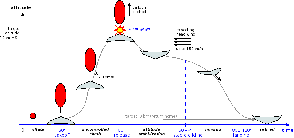
Figure 1: Mission plan
The goal of this project is to send a probe to the stratosphere and return it to the takeoff location. The probe consists of a flight controller with several sensors and is embedded into a styrowing glider. The glider is lightweight and able to perform basic flight maneuvers. In order to perform the mission, which is illustrated in Figure 1, the glider will be attached to a helium balloon, which will start ascending when released. Once it reaches its target altitude, the balloon is cut-off and the glider will fall. In this moment, the flight controller takes over control and autonomously navigates the glider back to its starting position on the ground. The hardware concepts for ascending and descending of the balloon and the probe itself have been developed by Matthias Jungmann in his diploma thesis.
Micro Glider
The micro glider is a styrowing that uses two servos to control the “elevons” (a mix-word of “elevator” and “aileron”) which are movable surfaces to control the flight behavior.
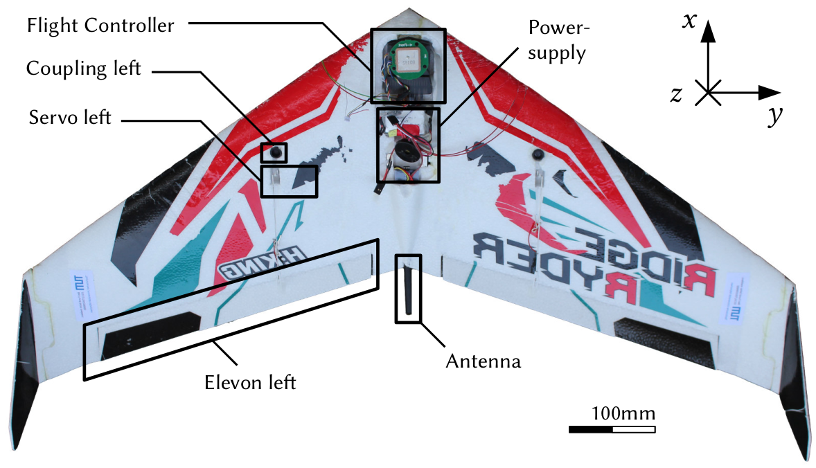
Photo of our high-altitude micro glider and important system components.
Flight Controller Theory
A flight controller performs several tasks which include monitoring and stabilization of an air vehicle. It reads sensors to obtain position and orientation of the vehicle and then computes the commands for the actuators that are required to keep the vehicle in a stable and controllable state. Modern flight controller for micro air vehicles are also responsible for navigation and guidance. Since our goal is stabilization and navigation of a styrowing, we will explain the theory of sensor fusion, control loops, and the GPS that are necessary for the software development.
Kalman-Filter
Pose estimation from sensor measurements is one major task for flight control. The linear filter described by R. Kálmán in 1960 1 allows optimal estimates of unknown variables measured by sensors with Gaussian noise. It is one of the most important algorithms for sensor fusion and used in a large variety of applications 2. The algorithm is used to estimate the value of a state variable and consists of two major calculation steps: (1.) prediction of the new state and (2.) updating the state estimation with measurement values. The equations in the following are derived from 2.
State Space Suppose we have the following state space model:
$$\vec{x}_{n} = \ma G_n \vec{x}_{n-1} + \ma B \vec{u}_n + \vec{v}_n$$
$$\vec{y}_{n} = \ma H_{n} \vec{x}_{n-1} + \vec{w}_{n}$$
with the state vector $\vec x$, transition matrix $\ma G$, Gaussian process noise $\vec v_n$, input vector $\vec u$, measurement vector $\vec y$, measurement model $\ma H$, and Gaussian measurement noise $\vec w_n$ at each discrete point in time $n \in \N$. The transition matrix represents the linear dynamic model, commonly based on physical laws.
1. Prediction: the prediction of the next state $\hat {\vec x}_{n|n-1}$ is based on the old state and the linear dynamic model $\ma G_n$. Additionally, the new process covariance $\ma C_{\vec x_{n|n-1}}$, which reflects the certainty of the model, is predicted with the dynamic model $\ma G_n$ and the process noise covariance $\ma C_{\vec v}$. $$\hat{\vec x}_{n|n-1} = \ma G_n \hat{\vec x}_{n-1|n-1} + \ma B \vec{u}_n$$
$$\ma C_{\vec x_{n|n-1}} = \ma G_n \ma C_{\vec x_{n-1|n-1}} \ma G_n^\top + \ma C_{\vec v}$$
2. Update: calculate the innovation $\Delta \vec y_n$, which is the difference between predicted and observed measurements. The certainty of measurement is expressed by the innovation covariance matrix $\ma S$, which depends on the measurement noise covariance matrix $\ma C_{\vec w_{n}}$. The innovation covariance matrix $\ma S$ is then used to calculate the Kalman gain matrix $\ma K_n$
$$\Delta \vec y_n = \vec y_n - \hat{\vec y}_{n|n-1} =\vec y_n - \ma H_{n} \hat{\vec x}_{n|n-1}$$ $$\ma S = \ma H_{n} \ma C_{\vec x_{n|n-1}} \ma H_{n}^\top + \ma C_{\vec w_{n}}$$ $$\ma K_n = \ma C_{\vec x_{n|n-1}} \ma H_{n}^\top {\ma S}^{-1}.$$
The Kalman gain matrix can be seen as the weights for $\Delta \vec y_n$. Its entries have the property $K_{ij} \in [0.0; 1.0],$ where 0.0 means the filter fully trusts the prediction and 1.0 means the filter fully trusts the measurement. Finally, the Kalman gain matrix is used to calculate the new state as well as its covariance matrix:
$$\hat{\vec x}_{n|n} = \hat{\vec x}_{n|n-1} + \ma K_n \Delta \vec y_n$$ $$\ma C_{\vec x_{n|n}} = \ma C_{\vec x_{n|n-1}} + \ma K_n \ma H_{n} \ma C_{\vec x_{n|n-1}}.$$
PID Controller
Real world control problems are often solved by a proportional-integral-derivative (PID) controller, which was invented in 1910 and gained popularity since then 3. It offers a very simple, yet efficient control scheme that is easy to implement in low-level software. The PID controller can compensate low frequencies, such as steady-state errors and also provides a good transient response 3. Its basic structure is illustrated in the figure below. The difference between the desired value $r(t)$ and the actual sensor measurement $y(t)$ is the control error $e(t)$. The PID controller takes proportional part (P), integral (I), and derivation (D) of the control error and calculates a weighted sum to generate a control output $u(t)$ for the actuators that manipulate the physical process.

Block diagram of a typical PID controller loop.
The output $u(t)$ of the PID controller can be formulated as
$$ u(t) = K_{\mathrm{P}} \cdot e(t) + K_{\mathrm{I}} \int\limits_{0}^{t} e(\tau) \diff \tau + K_{\mathrm{D}} \frac{\diff e(t)}{\diff t} , $$
with the gains $K_{\mathrm{P}}$, $K_{\mathrm{I}}$, $K_{\mathrm{D}}$, and the error $e(t) = r(t) - y(t)$. For a time discrete system, the derivation and integral can be approximated and the control equation for a point in time $t_i$ simplifies to
$$u[t_i] = K_{\mathrm{P}} \cdot e[t_i] + K_{\mathrm{I}} \sum\limits_{l = 1}^{i} e[t_l] (t_l - t_{l-1}) + K_{\mathrm{D}} \frac{e[t_i] - e[t_{i-1}]}{t_i - t_{i-1}}$$
The challenge in control theory is to find proper values for the gains. Especially the derivative part, which can increase control stability, is often difficult to tune 3.
Navigation and Guidance
“Navigation is the determination of the position and velocity of a moving vehicle” 4. In contrast, guidance is steering towards a destination. The flight controller needs to perform both navigation and guidance. For basic navigation and guidance, three terms are important: heading, course, and bearing. The heading is the direction a vehicle is pointing. The course is the intended heading from a start point to a target point. The absolute bearing is the clockwise angle between north and the line from the vehicle’s own position to its target position. The relation of these terms is illustrated in the figure below. If there were no external influences, such as wind, the bearing, the course, and the heading would be the same. However, in a realistic scenario, the aircraft is drifting and as a result the bearing is deviating from the course, which must be compensated by controlling the heading.

Important angles for the navigation of the glider.
Bearing The bearing $\theta$ of an aircraft can be calculated from its own geographic position $(\varphi_1, \lambda_1)$ and its target geographic position $(\varphi_2, \lambda_2)$ by the equation
$$\theta = \arctan 2 \big( \sin( \Delta \lambda) ⋅ \cos (\varphi_2), \quad \cos(\varphi_1) ⋅ \sin(\varphi_2) - \sin(\varphi_1) ⋅ \cos(\varphi_2) ⋅ \cos (\Delta \lambda) \big)$$
where $\varphi$ is latitude, $\lambda$ is the longitude, and $\Delta \lambda = \lambda_2 - \lambda_1$. All angles are in radians.
Distance The distance between two locations can be calculated in several ways. The shortest distance is the line on the great-circle that connects the two points.
The equation Spherical Law of Cosines is the most precise and straight forward method, however, it is only numerical stable at a precision of IEEE-754 64bit floating-point numbers 5.
For short distances with small differences between longitude ($\approx 1,\deg$), a simple Pythagoras approximation is numerically stable and fast. However, for a good compromise, the haversine formula seemed to be adequate. It takes the spherical shape of the earth into account and is numerical stable 5. The distance $d$ is calculated by the haversine equations as
$$a = \sin^2\left(\frac{\Delta \varphi}{2}\right) + \cos(\varphi_1) \cdot \cos(\varphi_2) ⋅ \sin^2\left(\frac{\Delta \lambda}{2}\right)$$ $$d = 2 \cdot R_{\mathrm{Earth}} \cdot \arctan 2 \left( \sqrt{a}, \sqrt{1-a} \right)$$
where $\varphi$ is the latitude, $\lambda$ the longitude, and $R_{\mathrm{Earth}}$ the radius of the earth.
Flight Stack Software
Safety Concepts
In order to prevent failure of the software, we have selected several safety concepts that were applied during the development process. Since the general safety goal is to prevent errors as early as possible, there are concepts for each development phase beginning at the requirement specification phase. All concepts shall help to either avoid, detect, or mitigate fault, errors, and failures

Software Architecture.
Software Architecture
As illustrated in the figure above, the architecture was divided in 5 hierarchical layers with the top-down order: Tasks, Modules, Device Managers, Device Drivers, and \gls{HAA}. Additional required algorithms that have no further dependencies are packed into libraries which are not part of the hierarchy. A software unit in one hierarchical layer is only allowed to make calls to units in a lower layer, to libraries, or to units in the same layer if no cyclic dependencies are created.
Tasks: run multi-threaded on the CPU. The Ravenscar runtime schedules the tasks and ensures that no blocking can occur. Our application was planned to consist of only one mission task that is responsible for the overall behavior of the styrowing. It runs a FSM that represents the different states of the mission such as ascent and descent.
Modules: provide encapsulation of the main functionality. They group together related subprograms and represent a coherent part of the software. Each module can handle one or more device managers and provides a more abstract interface towards the mission task. We divided the application in 3 main modules: Estimator, Controller, and Logger.
Flight Test
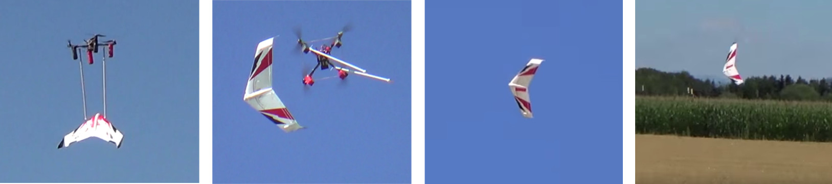
Drop test using a drone.
References
-
R. E. Kalman, “A new approach to linear filtering and prediction problems”, Transactions of the ASME–Journal of Basic Engineering, vol. 82, no. Series D, pp. 35–45, 1960. doi: 10.1115/1.3662552. ↩︎
-
R. Faragher, “Understanding the basis of the kalman filter via a simple and intuitive derivation”, IEEE Signal Processing Magazine, vol. 29, no. 5, pp. 128–132, Sep. 2012, issn: 1053-5888. doi: 10.1109/MSP.2012.2203621. ↩︎
-
K. H. Ang, G. Chong, and Y. Li, “Pid control system analysis, design, and technology”, IEEE Transactions on Control Systems Technology, vol. 13, no. 4, pp. 559–576, Jul. 2005, issn: 1063-6536. doi: 10.1109/TCST.2005.847331. ↩︎
-
M. Kayton and W. R. Fried, Avionics Navigation Systems. May 1997, ISBN: 978-0-471-54795-2 ↩︎
-
C. Veness. (2002). Calculate distance, bearing and more between latitude/longitude points, [Online]. Available: http://www.movable-type.co.uk/scripts/latlong.html (visited on 10/22/2016). ↩︎